blog

EAsT: Embeddings As Teachers for Music Classification

by Yiwei Ding

Due to the increasing use of neural networks, the last decade has seen dramatic improvements in a wide range of music classification tasks. However, the increased algorithmic complexity of the models requires an increased amount of data during the training process. Therefore, transfer learning is applied where the model is first pre-trained on a large-scale dataset for the source tasks and then fine-tuned with a comparably small dataset of the target task. T However, the increasing model complexity also makes the inference computationally expensive, so knowledge distillation is proposed where a low-complexity (student) model is trained while leveraging the knowledge in the high-complexity (teacher) model.

In this study, we integrate ideas and approaches from both transfer learning and knowledge distillation and apply them to the training of low-complexity networks to show the effectiveness of knowledge transfer for music classification tasks. More specifically, we utilize pre-trained audio embeddings as teachers to regularize the feature space of low-complexity student networks during the training process.

Methods

flow chart
Overall pipeline of training a model by using pre-trained embeddings as teachers. The training loss is a weighted sum (weighting factor omitted in the figure) of prediction loss and regularization loss. The regularization loss measures the distance between pre-trained embedding and the output feature map after the feature alignment. During inference, only the bottom part with the blue background is used.

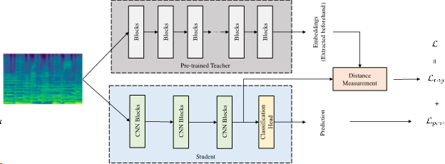
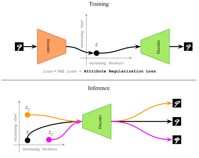
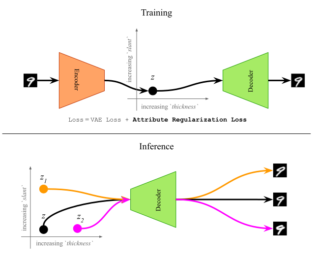
Similar to knowledge distillation, we rewrite our loss function as a combination of cross entropy loss for the classification task and a regularization loss that measures the distance between the student network’s feature map and the pre-trained embeddings with two different distance measures.

Experiments

We test the effectiveness of using pre-trained embeddings as teachers on two tasks: musical instrument classification with OpenMIC and music auto-tagging with MagnaTagATune, and we use four different embeddings: VGGish, OpenL3, PaSST and PANNs.

The following systems are evaluated for comparison:
• Baseline: CP ResNet (on OpenMIC) and Mobile FCN (on MagnaTagATune) trained without any extra regularization loss.
• TeacherLR: logistic regression on the pre-trained embeddings (averaged along the time axis), which can be seen as one way to do transfer learning by freezing the whole model except for the classification head.
• KD: classical knowledge distillation where the soft targets are generated by the logistic regression.
• EAsTCos-Diff: feature space regularization that uses cosine distance difference and regularizes only the final feature map.
• EAsTFinal and EAsTAll: proposed systems based on distance correlation as the distance measure, either regularizing only at the final stage or at all stages, respectively.
• EAsTKD: a combination of classical knowledge distillation and our method of using embeddings to regularize the feature space. The feature space regularization is done only at the final stage.

Results

results
Results on OpenMIC (above) and MagnaTagATune (below) datasets for different models regularized with different pre-trained embeddings. Best performances are in bold, and best results excluding the teachers are underlined.

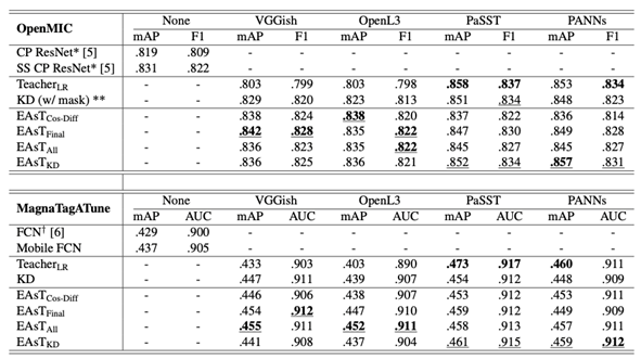
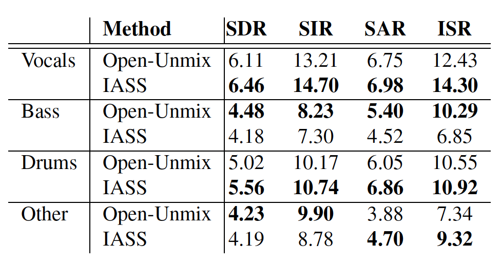
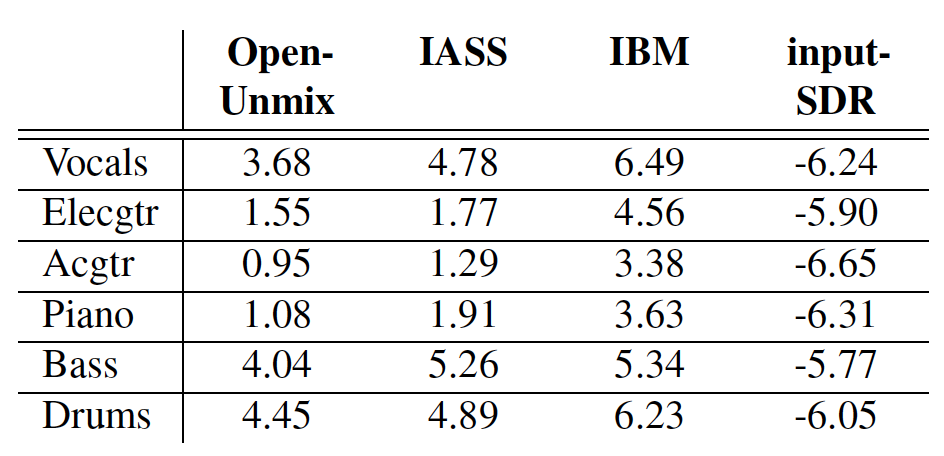
Table 1 shows the results on the OpenMIC and the MagnaTagATune dataset. We can make the following observations:
• Models trained with the extra regularization loss consistently outperform the non-regularized ones on both datasets, with all features and all regularization methods.
• Whether the teachers themselves have an excellent performance (PaSST and PANNs) or not (VGGish and OpenL3), students benefit from learning the additional knowledge from these embeddings, and the students’ upper limit is not bounded by the performance of teachers.
• As for the traditional knowledge distillation, the models perform best only with a “strong” teacher like PaSST and PANNs, which means the method is dependent on high-quality soft targets generated by the “strong” teachers.
• The combination system EAsTKD gives us better results with PaSST and PANNs embeddings while for VGGish and OpenL3 embeddings, the performance is not as good as EAsTFinal or EAsTAll in most cases.

model complexity
Comparison of the model complexity

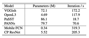
Table 2 lists the number of parameters as well as rough inference speed measurements of the models. We can see that Mobile FCN and CP ResNet are much faster in inference than pre-trained models.

Conclusion

In this study, we explored the use of audio embeddings as teachers to regularize the feature space of low-complexity student networks during training. We investigated several different ways of implementing the regularization and tested its effectiveness on the OpenMIC and MagnaTagATune datasets. Results show that using embeddings as teachers enhances the performance of the low-complexity student models, and the results can be further improved by com bining our method with a traditional knowledge distillation approach.

Resources

• Code: The code for reproducing experiments is available in our Github repository.
• Paper: Please see the full paper for more details on our study.

Latte: Cross-framework Python Package for Evaluation of Latent-Based Generative Models

by Karn N. Watcharasupat and Junyoung Lee

Controllable deep generative models have promising applications in various fields such as computer vision, natural language processing, or music. However, implementations of evaluation metrics for these generative models remain non-standardized. Evaluating disentanglement learning, in particular, might require implementing your own metrics, possibly entangling you more than when you started.

Latte (for latent tensor evaluation) is a package designed to help both you and your latent-based model to stay disentangled at the end of the day (YMMW, of course). The Python package is, by design, created to work with both PyTorch and TensorFlow. All metrics are first implemented in NumPy with minimal dependencies (like scikit-learn) and then a wrapper is created to turn these NumPy functions into TorchMetrics or Keras Metric modules. This way, each metric is always calculated in the exact same way regardless of the deep learning framework being used. In addition, the functional NumPy API is also exposed, so that post-hoc evaluation or models from other frameworks can also enjoy our metric implementations.

Currently, our package supports the classic disentanglement metrics: Mutual Information Gap (MIG), Separate Attribute Predictability (SAP), Modularity. In addition, several dependency-aware variants of MIG proposed here and here are also included. These metrics are useful for situations where your semantic attributes are inherent dependent with respect to one another, a situation where traditional metrics might penalize a latent space that has correctly learned the nature of the semantic attributes. Latte also implements interpolatability metrics which evaluate how smoothly or monotonically your decoder translates the latent vectors into generated samples.

To make life simpler, Latte also comes equipped with metric bundles which are optimized implementations of multiple metrics commonly used together. The bundles optimize away duplicate computation of identical or similar steps in the metric computation, reducing both the lines of code needed and the runtime. We are working to add more metrics and bundles into our package. The most updated list can always be found at our GitHub repository.

Latte can be easily installed via pip using pip install latte-metrics. We have also created a few Google Colab notebooks demonstrating how you can use Latte to evaluate an attribute-regularized VAE for controlling MNIST digits, using vanilla PyTorch, PyTorch Lightning, and TensorFlow. The full documentation of our package can be found here.

Resources

Score-Informed Networks for Music Performance Assessment

by Jiawen Huang and Yun-Ning Hung

Learning to play a musical instrument usually requires continuing feedback from a trained professional to guide the learning process. Although reduced face-time with a teacher might make instrument learning more accessible, it also slow the learning process down. An automatic music performance assessment system, however, might fill this gap by providing instant and objective feedback to the student during practice sessions.

Figure 1: Score-informed Music Performance Assessment

Some of the previous research extract features from both the performance audio and the score. With the rise of deep learning, neural networks replaced traditional feature extraction. However, the vast majority of previous studies focus on the audio information and ignore the score information. This, however, discards a significant amount of arguably important side information that could be utilized for assessing the student performance.

In this work, we explore different methods to incorporate musical score information into deep-learning models for music performance assessment. Our hypothesis is that including this information will lead to improved performance of deep networks for this task. More specifically, we present three architectures which combine score and audio inputs to make a score-informed assessment of a music performance. We refer to these three architectures as Score-Informed Network, Joint Embedding Network and Distance Matrix Network. The input of all three networks is based on the extracted fundamental frequency contour converted to pitches.

Score-Informed Network (SIConvNet)

Figure 2: Architecture of SIConvNet

The input representation for SIConvNet is constructed by stacking an aligned pitch contour and score pair to create a N × 2 matrix. The matrix is then fed into 4-layer 1-D convolutional layers followed by a linear layer, as shown in Figure 2.

Joint Embedding Network (JointEmbedNet)

Figure 3: Architecture of JointEmbedNet

The second approach is based on the assumption that performances are rated based on perceived distance between the performance and the underlying score being performed. The individual N × 1 sequences are fed separately into two encoders to project the score and the pitch contour to a joint latent space. Then, we use the cosine similarity cos⁡(Escore, Eperformance) between the two embeddings to obtain the predicted assessment rating.

Distance Matrix Network (DistMatNet)

Figure 4: Architecture of DistMatNet

The final approach assumes that given the information from both the pitch contour and the score, the task of performance assessment can be interpreted as finding a performance distance between them. As a result, we use a distance matrix between the pitch contour and the score as the input to the network to learn the pitch difference. A deep residual architecture with two linear layers is used to perform assessment score prediction.

Experiments

The dataset we use is a subset of a large dataset of middle school and high school student performances recorded for the Florida All State Auditions. The recordings contain auditions spanning 6 years (from 2013 to 2018), featuring several monophonic pitched and percussion instruments, and include several exercises. In this experiment, we limit ourselves to the technical etude for middle school and symphonic band auditions. We choose Alto Saxophone, Bb Clarinet, and Flute performances due to these being the most populated instrument classes. Each performance is rated on a point-based scale by one expert along 4 criteria defined by the Florida Bandmasters’ Association (FBA): (i) musicality, (ii) note accuracy and (iii) rhythmic accuracy. As a result, all the models mentioned above are trained to predict the regression ratings (which are normalized between 0 and 1) given by the experts.

Results

Figure 5: Results (Rsquared) for Middle School (left) and Symphonic Band (right)

We compared our methods with the baseline (score-independent) model in our previous work. The results show that:

  • Although all score-informed models generally outperform the baseline, the difference between baseline and score-informed models is smaller for the middle school. This implies that a score reference becomes more impactful with increasing proficiency level.
  • All systems perform better (higher R2 value) on the middle school recordings than on the symphonic band recordings. Possible explanation is that symphonic band scores are usually more complicated and longer. Furthermore, symphonic band auditions might exhibit greater skill level than middle school performers, which could complicate modeling the differences.
  • While the two models SIConvNet and JointEmbedNet both use the same input features, JointEmbedNet outperforms SIConvNet in most of the experiments. We can assume that JointEmbedNet is able to explicitly model the differences between the input pitch contour and score.
  • While both DistMatNet and JointEmbedNet utilize the similarity between the score and pitch contour, JointEmbedNet typically performs better across categories and bands.

Conclusion

This work presents three novel neural network-based methods that combine score information with a pitch representation of an audio recording to assess a music performance. The results show a considerable improvement over the baseline model. One shortcoming of the investigated models is that they are agnostic to timbre and dynamics information, which might be critical factors in performance assessment. We leave this area for future research.

Resources

  • Code: The code for reproducing experiments is available in our Github repository.
  • Paper: Please see the full paper for more details on our study.

Multi-Task Learning for Instrument Activation Aware Music Source Separation

by Yun-Ning Hung

Motivation

Music source separation performance has been improved dramatically in recent years due to the rise of deep learning, especially in the fully-supervised learning setting. However, one of the main problems of the current music source separation systems is the lack of large-scale datasets for training. Most of the open-source datasets either have limited size, or the number of included instruments and music genres is limited.

Moreover, many existing systems focus exclusively on the problem of source separation itself and ignore the utilization of other possibly related MIR tasks which could lead to additional quality gain.

In this research work, we leverage two open-source large-scale multi-track datasets, MedleyDB and Mixing Secrets, in addition to the standard MUSDB to evaluate on a large variety of separable instruments. We also propose a multitask learning structure to explore the combination of instrument activity detection and music source separation. The goal is that by training these two tasks in an end-to-end manner, the estimated instrument labels can be used during inference as a weight for each time frame. We refer to our method as instrument aware source separation (IASS).

Model structure

Figure 1: Multitask model structure for our proposed source separation system.

Our proposed model is a U-net based structure with residual blocks instead of CNNs at each layer. The reason for choosing the U-net structure is that it has been found useful in image decomposition, a task with general similarities to source separation. The residual block allows the information from the current layer to be fed into a layer 2 hops away and deepens the structure. A classifier is attached to the latent vector to predict the instrument activity. Mean Square Error (MSE) loss is used for source separation while Binary Cross-Entropy (BCE) loss is used for instrument activity prediction.

Instrument weight

Figure 2: Using instrument activation as a weight to filter the estimated mask, which will be used to multiply with the mixture of the magnitude spectrogram.

We use instrument activation as a weight to multiply with the estimated mask along the time dimension. By doing so, the instrument labels are able to suppress the frames not containing any target instrument. The instrument activation is first binarized by using a threshold. A median filter is then applied to smooth the estimated activation.

Experiments & Results

We compare our model with baseline Open-Unmix model. Both models use mixture phase without any post-processing. We train and evaluate both models on two datasets, MUSDB-HQ dataset and the combination of Mixing Secrets and MedleyDB.

Figure 3: BSS metrics for Open-Unmix and IASS on the MUSDB-HQ dataset.

The result shows that when training and evaluating on the MUSDB-HQ dataset, our model outperforms the Open-Unmix model on ‘Vocals’ and ‘Drums’, performs equally on ‘Other’, and slightly worse on ‘Bass’. This might be because ‘Bass’ is likely to appear throughout the songs; as a result, the improvement of using the instrument activation weight is limited.

Figure 4: SDR score for Open-Unmix, IASS, an ideal binary mask and input-SDR.

Figure 4 summarizes the results for the combination of the MedleyDB and Mixing Secrets datasets. The Ideal Binary Mask (IBM) represents the best-case scenario. The worst-case scenario is represented by the results for input-SDR, which is the SDR score when using the unprocessed mixture as the input. We can observe that our model also outperforms Open-Unmix on all the instruments. Moreover, both models have higher scores on ‘Drums,’ ‘Bass,’ and ‘Vocals’ than on ‘Electrical Guitar’, ‘Piano’, and ‘Acoustic Guitar’. This might be attributed to the fact that ‘Guitar’, ‘Piano’, and ‘Acoustic Guitar’ have fewer training samples. Another possible reason is that the more complicated spectral structure of polyphonic instruments such as ‘Guitar’ and ‘Piano’ make the separation task more challenging.

Conclusion

This work presents a novel U-net based model that incorporates instrument activity detection with source separation. We also utilize a larger dataset to evaluate various instruments. The result shows our model achieves equal or better separation quality than the baseline model. Future extension of this work includes:

  • Increasing the amount of data by using a synthesized dataset,
  • Incorporating other tasks, such as multi-pitch estimation, into our current model, and
  • Exploring post-processing methods such as Wiener filter, to improve our system’s quality.

Resources

  • The code for reproducing experiments is available on our Github repository.
  • Please see the full paper (to appear in ISMIR ’20) for more details on the dataset and our experiment.

AR-VAE: Attribute-based Regularization of VAE Latent Spaces

by Ashis Pati

In the context of deep generative models, improving controllability by enabling selective manipulation of data attributes has been an active area of research. Latent representation-based models such as Variational Auto-Encoders (VAEs) have shown promise in this direction as they are able to encode certain hidden attributes of the data.

In this research work, we propose a supervised training method which uses a novel regularization loss to create structured latent spaces where specific continuous-valued attributes are forced to be encoded along specific dimensions of the latent space. For instance, if the attributes represents ‘thickness’ of a digit, and the regularized dimensions correspond to the first dimension of the latent space, then sampling latent vectors with increasing values of the first dimension should result in the same digit with increased thickness. This overall idea is shown in Figure 1 below. The resulting Attribute-Regularized VAE (AR-VAE) can then be used to manipulate these attributes by simple traversals along the regularized dimension.

Figure 1: Overall schematic of the AR-VAE model.

AR-VAE has several advantages over previous methods. Unlike Fader Networks it is designed to work with continuous-valued attributes, and unlike GLSR-VAE, it is agnostic to the way attributes are computed or obtained.

Method

In order to create a structured latent space where an attribute $a$ is encoded along a dimension $r$, we add a novel attribute regularization loss to the standard VAE-objective. This loss is designed such that as we traverse along $r$, the attribute value $a$ of the generated data increases. To formulate the loss function, we consider a mini-batch of $m$ examples, and follow a three-step process:

1. Compute an attribute distance matrix $D_a$
2. Compute a regularized dimension distance matrix $D_r$
3. Compute the mean absolute error between signs of $D_a$ and $D_r$

In practice, we compute the hyperbolic tangent of $D_r$ so as to ensure differentiability of the loss function with respect to the latent vectors. Multiple regularization terms can be used to encode multiple attributes simultaneously. For a more detailed mathematical description of the loss function, check out the full paper.

Experimental Results

We evaluated AR-VAE using different datasets from the image and music domains. Here, we present some of the results of manipulating different attributes. For detailed results on other experiments such as latent space disentanglement, reconstruction fidelity, content preservation, and hyperparameter tuning, check out the full paper.

Manipulation of Image Attributes

Manipulating attributes of 2-d shapes. Each row in the figure below represents a unique shape (from top to bottom): square, heart, ellipse. Each column corresponds to traversal along a regularized dimension which encodes a specific attribute (from left to right): Shape, Scale, Orientation, x-position, y-position.


Manipulating attributes of MNIST digits. Each row in the figure below represents a unique digit from 0 to 9. Each column corresponds to traversal along a regularized dimension which encodes a specific attribute (from left to right): Area, Length, Thickness, Slant, Width, Height.


Manipulation of Musical Attributes

Manipulating attributes of monophonic measures of music. In the figure below, measures on each staff line are generated by traversal along a regularized dimension which encodes a specific musical attribute (shown on the extreme left).

Piano-roll version of the figure above is shown below. Plots on the right of each piano-roll show the progression of attribute values.

Conclusion

Overall, AR-VAE creates meaningful attribute-based interpolations while preserving the content of the original data. In the context of music, it can be used to build interactive tools or plugins to aid composers and music creators. For instance, composers would be able to manipulate different attributes (such as rhythmic complexity) of the composed music to try different ideas and meet specific compositional requirements. This would allow fast iteration and would be especially useful for novices and hobbyists. Since the method is agnostic to how the attributes are computed, it can potentially be useful to manipulate high-level musical attributes such as tension and emotion. This will be particularly useful for music generation in the context of video games where the background music can be suitably changed to match the emotional context of the game and the actions of the players.

Resources

dMelodies: A Music Dataset for Disentanglement Learning

by Ashis Pati

Motivation

In the field of machine learning, it is often required to learn low-dimensional representations which capture important aspects of given high-dimensional data. Learning compact and disentangled representations (see Figure 1) from given data, where important factors of variation are clearly separated, is considered especially useful for generative modeling.

Figure 1: Disentangled representation learning.

However, most of the current/previous studies on disentanglement have relied on datasets from the image/computer vision domain (such as the dSprites dataset).

We propose dMelodies, a standardized dataset for conducting disentanglement studies on symbolic music data which will allow:

  • researchers working on disentanglement algorithms evaluate their method on diverse domains.
  • systematic and comparable evaluation of methods meant specifically for music disentanglement.

dMelodies Dataset

To enable objective evaluation of disentanglement algorithms, one needs to either know the ground-truth values of the underlying factors of variation for each data point, or be able to synthesize the data points based on the values of these factors.

Design Principles

The following design principles were used to create the dataset:

  • It should have a simple construction with homogeneous data points and intuitive factors of variation.
  • The factors of variation should be independent, i.e., changing any one factor should not cause changes to other factors.
  • There should be a clear one-to-one mapping between the latent factors and the individual data points.
  • The factors of variation should be diverse and span different types such as discrete, ordinal, categorical and binary.
  • The generated dataset should be large enough to train deep neural networks.
Dataset Construction

Based on the design principles mentioned above, dMelodies is artificially generated dataset of simple 2-bar monophonic melodies generated using 9 independent latent factors of variation where each data point represents a unique melody based on the following constraints:

  • Each melody will correspond to a unique scale (major, harmonic minor, blues, etc.).
  • Each melody plays the arpeggios using the standard I-IV-V-I cadence chord pattern.
  • Bar 1 plays the first 2 chords (6 notes), Bar 2 plays the second 2 chords (6 notes).
  • Each played note is an 8th note.

A typical example is shown below in Figure 2.

Figure 2: Example melody from the dMelodies dataset along with the latent factors of variation.


Factors of Variation

The following factors of variation are considered:

1. Tonic (Root): 12 options from C to B
2. Octave: 3 options from C4 through C6
3. Mode/Scale: 3 options (Major, Minor, Blues)
4. Rhythm Bar 1: 28 options based on where the 6 note onsets are located in the first bar.
5. Rhythm Bar 2: 28 options based on where the 6 note onsets are located in the second bar.
6. Arpeggiation Direction Chord 1: 2 options (up/down) based on how the arpeggio is played
7. Arpeggiation Direction Chord 2: 2 options (up/down)
8. Arpeggiation Direction Chord 3: 2 options (up/down)
9. Arpeggiation Direction Chord 4: 2 options (up/down)

Consequently, the total number of data-points are 1,354,752.

Benchmarking Experiments

We conducted benchmarking experiments using 3 popular unsupervised algorithms (beta-VAE, Factor-VAE, and Annealed-VAE) on the dMelodies dataset and compared the result with those obtained using the dSprites dataset. Overall, we found that while disentanglement performance across different domains is comparable (see Figure 3), maintaining good reconstruction accuracy (see Figure 4) was particularly hard for dMelodies.

Figure 3: Disentanglement performance (higher is better) in terms of Mutual Information Gap (MIG) of different methods on the dMelodies and dSprites datasets.


Figure 4: Reconstruction accuracies (higher is better) of the different methods on the dMelodies and dSprites datasets. For reconstruction, the median accuracy for 2 methods fails to cross 50% which makes them unusable in a generative modeling setting.


Thus, methods which work well for image-based datasets do not extend directly to the music domain. This showcases the need for further research on domain-invariant algorithms for disentanglement learning. We hope this dataset is a step forward in that direction.

Resources

The dataset is available on our Github repository. The code for reproducing our benchmarking experiments is available here. Please see the full paper (to appear in ISMIR ’20) for a more in-depth discussion on the dataset design process and additional results from the benchmarking experiments.


Learning to Traverse Latent Spaces for Musical Score Inpainting

Inpainting as a Creative Tool

Inpainting is the task of automatically filling in missing information in a piece of media (say, an image or a audio clip). Traditionally inpainting algorithms have been used mostly for restorative purposes. However, in many cases, there could be multiple ways to perform an inpainting task. Hence, inpainting algorithms can be used as a creative tool.

Figure 1:

Specifically for music, an inpainting model could be used for several applications in the field of interactive music creation such as:

  • to generate musical ideas in different styles,
  • to connect different musical sections, and
  • to modify and extend solos.

Motivation

Previous work, e.g., Roberts et al.’s MusicVAE, has shown that Variational Auto-Encoder (VAE)-based music generation models show interesting properties such as interpolation and attribute arithmetic (this article gives an excellent overview of these properties). Effectively, for music, we can train a low-dimensional latent space where each point maps to a measure of music (see Fig. 3 for an illustration).

Figure 2:

Now while linear interpolation in latent spaces has shown interesting results, by definition, it cannot model repetition in music (joining two points in euclidean space with a line will never contain the same point twice). The key motivation behind this research work was to explore if we can learn to traverse complex trajectories in the latent space to perform music inpainting, i.e., given a sequence of points corresponding to the measures in the past and future musical contexts, can we find a path through this latent space which can form a coherent musical sequence (see Fig. 4).

Figure 3:

Method

To formalize the problem, consider a situation where we are given the beginning and end of a song (which we refer to as the past musical context Cp and future musical context Cf, respectively) The task here is to create a generative model which connects the two contexts in a musically coherent manner by generating an inpainting Ci. We further constrain the task by assuming that the contexts and the inpainting have a certain number of measures (see Fig. 2 for an illustration). So effectively, we want to train a generative model which can maximize the likelihood of p(Ci|Cp, Cf).

Figure 4:

In order to achieve the above objective, we train recurrent neural networks to learn to traverse the latent space. This is accomplished using the following steps:

    • We first train a MeasureVAE model to reconstruct single measures of music. This creates our latent space for individual measures.
Figure 5:
    • The encoder of this model is used to obtain the sequence of latent vectors (Zp and Zf) corresponding to the past and future musical contexts.
Figure 6:
    • Next, we train a LatentRNN model which takes these latent vector sequences as input and learns to output another sequence of latent vectors Zi corresponding
      Figure 7:

      to the inpainted measures.

    • Finally we use the decoder of the MeasureVAE to maps these latent vectors back to the music space to obtain our inpainting (Ci).
Figure 8:

More details regarding the model architectures and the training procedures are provided in our paper and our GitHub repository.

Results

We trained and tested our proposed model on monophonic melodies in the Scottish and Irish style. For comparison, we used the AnticipationRNN model proposed by Hadjeres et al. and a variant of it based our stochastic training procedure. Our model was able to beat both the baselines in objective test aimed at testing how well the model is able to reconstruct missing measures in monophonic melodies.

Figure 9:

We also conducted a subjective listening by asking human listeners to rate pairs of melodic sequences. In this our proposed model performed comparably to the baselines.

Figure 10:

While the method works fairly well, there were certain instances where the model produces pitches which are out of key. We think these “bad” pitch predictions were instrumental in reducing the perceptual rating of the inpaintings in the subjective listening test. This needs additional investigation. Interested readers can listen to some of these example inpaintings performed by our model in the audio examples list.

Overall, the method demonstrates the merit of learning complex trajectories in the latent spaces of deep generative models. Future avenues of research would include adapting this framework for polyphonic and multi-instrumental music.

Resources

An Attention Mechanism for Musical Instrument Recognition

Musical instrument recognition continues to be a challenging Music Information Retrieval (MIR) problem, especially for songs with multiple instruments. This has been an active area of research for the past decade or so and while the problem is generally considered solved for individual note or solo instrument classification, the occlusion or super-position of instruments and large timbral variation within an instrument class makes the task more difficult in music tracks with multiple instruments.

In addition to these acoustic challenges, data challenges also add to the difficulty of the task. Most methods for instrument classification are data-driven, i.e., they infer or ‘learn’ patterns from labeled training data. This adds a dependence on obtaining a reliable and reasonably large training dataset for instrument classification.

Data Challenges in Instrument Classification

In previous work, we discussed briefly how there was a data problem in the task of musical instrument recognition or classification in the multi-instrument/multi-timbral setting. We utilized strongly labeled multi-track datasets to overcome some of the challenges. This enabled us to train deep CNN-based architectures with short strongly labeled audio snippets to predict fine-grained instrument activity with a time resolution of 1 second.

In retrospect we can claim that, although instrument activity detection remains the ultimate goal, current datasets are both too small in scale and terribly imbalanced in terms of both genre and instruments as shown in this figure.

Distribution of instruments in one dataset

The OpenMIC dataset released in 2018 addresses some of these challenges by curating a larger-scale, somewhat genre-balanced set of music with 20 instrument labels and crowdsourced annotations for both positive (presence) and negative (absence) classes. The catch is that the audio clips here are 10 seconds long and the labels are assigned to the entire clip, i.e., fine-grained instrument activity annotations are missing. Such a dataset is what we call ‘weakly labeled.’

Previous approaches for instrument recognition are not designed to handle weakly labeled long clips of audio. Most of them are trained to detect instrument activity at short time-scales, i.e., the frame level up to 3 seconds. The same task with weakly labeled audio is tricky since instruments that are labeled as present may be present only instantaneously and could be left undetected by models that average over time.

In our proposed method, we utilize an attention mechanism and multiple-instance learning (MIL) framework to address the challenge of weakly labeled instrument recognition. The MIL framework has been explored in sound event detection literature as a means to weakly labeled audio event classification, so we decided to apply the technique to instrument recognition as well.

Method Overview

In MIL, each data point is represented as a bag of multiple instances. In our case, each bag is a 10 second clip from the OpenMIC dataset. We divide the clip into 10 instances, each of 1 second. Each instance is represented by a 128-dimensional feature vector extracted using a pre-trained VGGish model. Thus, a clip input is 10×128 dimensional. As per the MIL framework, each bag is associated with a label. This implies that at least one instance in the bag is associated with the same label, we just don’t know which one. To learn in the MIL setting, algorithms perform a weighted sum of instance-level predictions to obtain the bag-level predictions. These predictions can be compared with the bag-level labels to train the algorithm. In our paper, we utilize learned attention weights for the aggregation of instance-level predictions.

attention model

Looking at the model architecture in the figure above, the model estimates instance-level predictions and instance-level attention weights. We estimate one weight per instance per instrument label. The weights are normalized across instances to sum to one, adding an interpretation of relative contribution each instance prediction has on the final clip-level prediction for a particular instrument.

Results

We compared this model architecture with mean pooling, recurrent neural networks, fully connected networks and binary random forests and found our attention-based model to outperform all the other methods, especially in terms of the recall. We also tried to visualize the attention weights and see if the model was focusing on relevant parts of the audio as it was supposed to.

Visualization of attention weights

As you can see in the above image, while this model is not very adept at localizing the instruments (in the first example, violin is actually in all instances, but model applies high weights only to a couple of instances), it does a good job at seeking out easy to classify instances and focuses weights on those.

Conclusion

In conclusion, we discuss the merits of weakly labeled audio datasets in terms of ease of annotation and scalability. In our opinion, it is important to develop methods capable of handling weakly labeled data due to the ease of annotation and therefore scalability of such datasets. To that end, we introduce the MIL framework and discuss the attention mechanism in brief. Finally, we show a visualization of how the attention weights provide some degree of interpretability to the model. Even though the model is not perfectly localizing the instruments, it learns to focus on relevant instances for final prediction.

The detailed paper can be found here.


Explicitly Conditioned Melody Generation

by Benjamin Genchel

The advent of modern deep learning has rapidly propelled progress and attracted interest in symbolic music generation, a research topic that encompasses methods of generating music in the form of sequences of discrete symbols. While a variety of techniques have been applied to tasks in this domain, the majority of approaches treat music as a temporal sequence of events and rely on Recurrent Neural Networks (RNNs), specifically the gated variants Long Short-Term Memory (LSTM) and Gated Recurrent Units (GRU), to model this sequence. These approaches generally attempt only to learn to predict the next note event(s) in a series given previous note event(s). While results from these types of models have been promising, they train on hard mode relative to human musicians, who rely on explicit, discretely classed information such as harmony, feel (e.g. swing, straight), phrasing, meter, and beat to organize and contextualize while learning.

Our study aims to investigate how deep models, specifically gated RNNs, learn when provided with explicit musical information, and further, how particular types of explicit information affect the learning process. We describe the results of a case study in which we compared the effects on musical output of conditioning an RNN-based model like those mentioned above with various combinations of a select group of musical features.

Specifically, we separate musical sequences into sequences of discrete pitch and duration values, and model each sequence independently with its own LSTM-RNN. We refer to these as Pitch-RNN and Duration-RNN respectively. Then we train a pair of these models using combinations of the following:

  • Inter Conditioning: the pitch generation network is provided with the corresponding duration sequence as input and vice versa.
  • Chord Conditioning: both the pitch and duration networks are provided with a representation of the current chord for each input timestep.
  • Next Chord Conditioning: both the pitch and duration networks are provided with a representation of the chord following the current chord for each input timestep.
  • Bar Position Conditioning: both the pitch and duration networks are provided with a discrete value representing the position within a surrounding bar of the current input token.

For a more clear picture of what we’re doing, check out this architecture diagram!

Data

We trained our models using two datasets (Bebop Jazz and Folk) of lead sheets (data extracted from musicXML files), as lead sheets provide a simplified description of a song that is already segmented into explicit components.

Evaluation

Evaluating generative music is a challenging and precarious task. In lieu of an absolute metric for quality, we characterize the outputs of each trained model using a set of statistical methods:

  • Validation NLL — The final loss achieved by a model on the validation set.
  • BLEU Score — a metric originally designed for machine translation, but deployed fairly commonly for judging sequence generation in general, BLEU score computes a geometric mean of the counts of matching N-grams (specifically 1, 2, 3, and 4-grams) between a set of ground truth data and a data set generated by a model. A BLEU score can be between 0 and 1, with 0 being nothing in common and 1 being everything in common (exactly matching).
  • MGEval — the MGEval toolbox, created by our own Li-Chia “Richard” Yang and Alexander Lerch, and described in an earlier blog post on this page, calculates KL-divergence and overlap scores between distributions of a number of music specific statistical features calculated for a set of ground truth data and generated data. These scores give an idea of how much generated data differs from the ground truth, and further provides insight into how they differ in musical terms.

Results

Validation NLL

The general trend observed was, perhaps unsurprisingly, that the more conditioning information used, the lower the final loss. Additionally, models trained with more conditioning learned faster than trained with less.

BLEU Score

Pitch models generally achieved a higher BLEU score with added conditioning factors, while Duration networks demonstrated the opposite trend — lower scores with added conditioning factors. The highest scoring pitch models had both chord and next chord conditioning, though models trained on the Bebop dataset seemed to generally perform better with current chord conditioning than next-chord conditioning, while models trained on the Folk dataset performed better with next-chord conditioning. The highest scoring duration models for both datasets had no-conditioning at all, and the next highest scoring models had only one conditioning factor.
While a BLEU score close to 1 might be ideal for machine translation, for artistic tasks like music generation where there is no right answer, a score that high hints at overfitting, and thus a lack of ability to generalize what it has learned and create novel melodies in unfamiliar contexts. While pitch models scored between .1 and .3, duration models scored from .5 to .9; that duration models with less conditioning scored higher than those with more may actually indicate that models with more conditioning generalized better, as their scores were closer to .5

MGEval

MGEval produces a lot of numbers — In our case, 66 for a single model (6 scores each for 11 MGEval metrics we used). We aggregated these results in a way that gives each individual conditioning factor a probability indicating its likelihood of contributing to higher performance. We split our 11 metrics into two categories, pitch-based, and duration-based, and performed this aggregation for each set:

In general, we observed that scores on MGEval metrics improve with the addition of conditioning features, but with these aggregation scores, we were able to ascertain (at a high level) which types of conditioning were affecting what. For both datasets, inter and chord conditioning had strong effects on pitch based features, with bar position conditioning a close third. However, for duration based features, it’s harder to determine. We can see here that for models trained on the Folk set, it’s a bit of a grab bag, but for models trained on the Bebop set, chord and bar position clearly contribute the most to success. This is perhaps due to the much simpler, and more repetitive rhythmic patterns found in Folk music as compared to Bebop Jazz music.

Conclusions

Solid takeaways from this study are that conditioning with chords is important not just for pitch prediction, but for duration prediction as well, though the usefulness of conditioning with the next chord vs. the current chord was harder to determine. More generally, we were also able to gain insight into the relative usefulness of our chosen conditioning set for pitch and rhythm based features. Additionally, we saw that the usefulness of particular features can also be genre dependent. Further investigation, along with a subjective evaluation via listening test is certainly worthwhile.

Check out our paper, the associated website, or the codebase for more details, audio samples, data and other information!

Music Informatics Group @ICML Machine Learning for Music Discovery Workshop

There will be 2 presentations by our group at the ICML Machine Learning for Music Discovery Workshop (ML4MD) this year:

  • Pati, Ashis; Lerch, Alexander: Latent Space Regularization for Explicit Control of Musical Attributes:
    Deep generative models for music are often restrictive since they do not allow users any meaningful control over the generated music. To address this issue, we propose a novel latent space regularization technique which is capable of structuring the latent space of a deep generative model by encoding musically meaningful attributes along specific dimensions of the latent space. This, in turn, can provide users with explicit control over these attributes during inference and thereby, help design intuitive musical interfaces to enhance creative workflows.
  • Gururani, Siddharth; Lerch, Alexander; Bretan, Mason: A Comparison of Music Input Domains for Self-Supervised Feature Learning:
    In music using neural networks to learn effective feature spaces, or embeddings, that capture useful characteristics has been demonstrated in the symbolic and audio domains. In this work, we compare the symbolic and audio domains, attempting to identify the benefits of each, and whether incorporating both of the representations during learning has utility. We use a self-supervising siamese network to learn a low-dimensional representation of three second music clips and evaluate the learned features on their ability to perform a variety of music tasks. We use a polyphonic piano performance dataset and directly compare the performance on these tasks with embeddings derived from synthesized audio and the corresponding symbolic representations.